I’m using this page to archive some of the useful content from our slack workspace conversations.
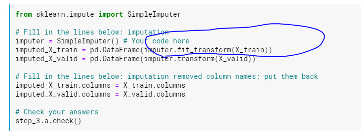
Why is fit_transform only here once?
A student asked me, in summary, what the whole “fit_transform” thing is here – isn’t fitting and transforming only for predictive models? They showed a snippet from one of the kaggle-learn courses.
Why is the training data hit with fit_transform?
This is a really key thing to learn about sklearn’s api, and why sklearn is just so so so much better than R for machine learning
Pretty much everything in sklearn, by convention, has to have a fit and fit_transform api, in order to be part of the sklearn family. Think broadly about a ML model from an abstract perspective–
First, a shell model is created. Nascent, empty, blank baby, but a shell nonetheless.
That’s commonly what happens whenever an instance of a sklearn class is instantiated – that’s the capital-letter class name called via ()
Ultimately, the goal is to use the new instance to do something. For a model, the goal is to make predictions. Before that can be done, the model / shell needs to be… fit. trained. Whatever synonym.
Only after it has been fit does it know how to do whatever it is it is going to be asked to do. In sklearn, you ask a… thing… to do something via calling transform on it
If you tried to call transform without having fit an instance, it will throw an exception (crash)
So, the fit_transform above is a convenience function, that both uses the training data to fit the imputer-machine. And then, and this is very important, anything you do to change the testing data, you have to do it to the training data, too. And to whatever else you’re going to ask your model to make predictions for in the future. Has to be mirrored. We’ll see more about that later.
The abstract thing to learn, is that imputers, onehotencoders, etc, all follow that paradigm. Fit it, then do something with it, to change the test/train data.
It’s not “fair” though to fit your machines on anything except the training data. No testing data allowed. To do otherwise is what is sometimes called “target leak.” The model shouldn’t, at any stage, have insight into the data it will be tested against.
One other thing from that snippet above. Sklearn is a punk in that it hates pandas-y things like column names. It uses, under the hood, numpy arrays, which coincidentally is the same thing that pandas builds on top of. So a lot of sklearn things can take a pandas df as input, but they’re jerks and will extract out the numpy array and only return a numpy array to you.
Or, it will transform it back into a pandas df before passing it back to you, but it doesn’t do the common courtesy of adding the columns back that it dropped. Jerks.
Now, what makes sklearn / python so much better for ML than R – it’s hat fit_transform api. everything has it. All possible modeling approaches. Which means it’s generally totally possible to try like a dozen different modeling approaches without needing to know specifics of how to call some library.
They’ll all have fit_transform. And they’ll all take a pandas df. That is not the case at all in R.
So, the SimpleImputer() in sklearn even though it only imputes the mean value of its current column into missing values of the same column needs to be “fit” to the training data? Why would the same function of imputation not throw a code on the validation data? I know it shouldn’t be fit to any form of testing but that itself is confusing me on why it’s required at all.
But with what value will it replace missing fields?
If the mean, then it has to memorize that value, to be used during the actual transforming. once it’s fit, the shell remembers it. It only has to be called once in the lifetime of a given class instantiation
The imputer object is updated in-place
With the sklearn approach, you don’t have to save the return value from fitting the object. The object itself is updated, you don’t need a new reference to the newly fitted object
Why is one hot encoding necesssary?
Q: I feel like this isn’t that complicated but I don’t really understand how one hot encoding helps improve a model
I too had this question once. It doesn’t improve anything, but a statistical model cannot deal with text – only numbers. It can only assign static weights that get multiplied by feature values.
What would .246 * blue be? .246 * red?
You might think to keep all the colors in the same column, and assign them number codes, but that only works if, say, blue (2) is
conceptually twice the amount of yellow (1), which of course doesn’t make sense. But since models can only assign one weight per
feature (column), that’s what it would be.
One hot encoding gives you one column/feature per string/factor value, so that the model can assign different weights to each value. And each column has either a 0 or a 1 value, so each factor level gets its own weight. And that weight is, for a
logistic regression, just the average of all values of the dependent variable that have the given factor level. (The
average in the presence of all other variables in the model).
And R does it for you (one hot encoding) as long as the feature is cast as type factor
Sklearn, you have to do it, but it’s easy enough to create a preprocessing pipeline that applies one hot encoding to each string columntype.
Can you go over PCA?
Student(s) comments in blockquotes, mine in plaintext.
we went over PCA in Advanced data analytics again and I’m just confused on it again
Have you ever looked at a 3d thing and drawn a 2d picture of it
If so, how many unique 2d pictures can you draw of a 3d thing – how did you choose the angle from which you would draw the 2d representation?
Lab deliverable: draw a 1,000 dimensional picture
Then draw a 2d version of the same
Your picture has to be a bunch of dots. The 2d angle perspective you choose has to screw up the placement of all of the dots the least. Like, it has to avoid ignoring interesting dimensional variations
Tell me if you are now enlightened
https://www.youtube.com/watch?v=FgakZw6K1QQ&t=168s YouTubeYouTube | StatQuest with Josh Starmer StatQuest: Principal Component Analysis (PCA), Step-by-Step
gimme 10 minutes
No! just based on my comments
absolutely not
the heck
they’re brilliant
sorry but I don’t draw things with dots
your paper begs to differ
lines are just a series of dots
I understand 3d in 2d by making dots bigger or smaller
? No, like go look at a car in real life
it’s 3d. now draw a picture of it on paper
the picture you draw depends on the angle from which you view the car
pretend that the car is made up of a bunch of dots. like as if it were on a television screen
mhm
that’s dimensionality reduction. PCA is a form of dimensionality reduction.
I get that
The “other part” is just choosing which angle to view the car from
That part is too confusing for a slack message
I think I understand (at least at a basic level) what it’s doing in terms of orthogonality. What causes my brain to glitch out is trying to interpret the code output. We ran some commands in class and it was just this huge block of stuff, and I had no idea how we were supposed to figure out which principle components were the most important
Ah. Can you paste some of the code output? Eigenvalues, right?
Something something keep retaining dimensions (components) as long as that component’s eigenvalue is greater than 1
   Standard deviations (1, .., p=9):
   [1] 1.7161519 1.2248362 1.1692700 1.0437981 0.9438854
   [6] 0.7085861 0.5957051 0.4655830 0.3650289
   Rotation (n x k) = (9 x 9):
                          PC1         PC2         PC3
   BEDS           -0.41873688  0.13319128 -0.35167055
   BATHS          -0.52874370  0.01534991 -0.12550822
   SQFT           -0.54357073  0.09832160 -0.02287134
   LOT.SIZE       -0.07570415  0.19432940  0.33824863
   YEAR.BUILT     -0.18033101 -0.20921633 -0.13484857
   PARKING.SPOTS  -0.41493506  0.16712524  0.34054911
   DAYS.ON.MARKET -0.04399613  0.19892730  0.73352157
   LATITUDE       -0.15919526 -0.64614726  0.18705810
   LONGITUDE       0.10917926  0.63703433 -0.19605564
                           PC4         PC5         PC6
   BEDS            0.342538737 -0.17860111  0.16930042
   BATHS          -0.085115982  0.03543441 -0.21473873
   SQFT            0.083416533 -0.08481286 -0.13379668
   LOT.SIZE       -0.393269387 -0.81941264  0.02773629
   YEAR.BUILT     -0.792118540  0.29894693 -0.15998079
   PARKING.SPOTS  -0.010723811  0.30599071  0.25308462
   DAYS.ON.MARKET  0.123762639  0.26983943 -0.13403500
   LATITUDE       -0.007631102 -0.06403547  0.67333253
   LONGITUDE      -0.266197574  0.16823290  0.58784866
                           PC7         PC8         PC9
   BEDS           -0.277109917  0.62755641 -0.18637761
   BATHS          -0.206883617 -0.56317012 -0.53839363
   SQFT           -0.009051483 -0.19966122  0.78888593
   LOT.SIZE        0.049971025  0.06683385 -0.09089431
   YEAR.BUILT     -0.141571145  0.36996761  0.07868799
   PARKING.SPOTS   0.687153132  0.15529298 -0.17271908
   DAYS.ON.MARKET -0.542215265  0.14222091 -0.01087676
   LATITUDE       -0.208270006 -0.13795469  0.04707962
   LONGITUDE      -0.219623829 -0.21078610  0.08021491
“eigenvalues”…. Now that’s a name I haven’t heard in a long time…
it’s a synonym to “krackenvalues”
  Call:
  lm(formula = LIST.PRICE ~ ., data = boulder.clean2)
  Residuals:
       Min       1Q   Median       3Q      Max
  -1502.36  -258.46   -27.44   198.96  3094.04
  Coefficients:
              Estimate Std. Error t value Pr(>|t|)
  (Intercept)  1170.18      34.11  34.305  < 2e-16 ***
  PC1          -378.28      19.92 -18.988  < 2e-16 ***
  PC2            72.10      27.91   2.583   0.0105 *
  PC3            94.06      29.24   3.217   0.0015 **
  PC4            28.37      32.75   0.866   0.3873
  PC5          -234.01      36.22  -6.461 7.26e-10 ***
  PC6          -498.20      48.25 -10.325  < 2e-16 ***
  PC7           126.18      57.39   2.199   0.0290 *
  PC8          -139.30      73.43  -1.897   0.0592 .
  PC9           815.45      93.66   8.706 9.74e-16 ***
  ---
  Signif. codes:
  0 '***' 0.001 '**' 0.01 '*' 0.05 '.' 0.1 ‘ ’ 1
  Residual standard error: 503.6 on 208 degrees of freedom
  Multiple R-squared:  0.746,	Adjusted R-squared:  0.735
  F-statistic: 67.88 on 9 and 208 DF,  p-value: < 2.2e-16
The second output is just output from a model where all columns have been replaced with PCA component scores
because that’s what we did
I think the first one shows how each of the columns “load” onto a given component
i’m guessing that the values at the top are eigenvalues?
something something loading. what command did you run that gave that output? It’s good form in sharing R code to have the first thing in the pasted output be the command run
prcomp(boulder.clean1, scale = TRUE)
any features / predictors that “load sufficiently” onto a PCA component can be said to be “represented” by that PCA component
Maybe the problem here is that we did not cover this using technical terms like eigenvalues and such. You’re asking us questions about things using terminology that was not covered in class (at least not in advanced analytics this morning)
but there’s an arbitrary rule that the absolute values of the loadings have to be greater than .7 IIRC
meaning all of those PCA components suck
ah i see. but look at that output you posted again, look at PC1:
four of the features “load” > .4. That group of features “represents” PC1
PC2, now look there. LATITUDE and LONGITUDE are massive. PC2 basically only represents those two (edited)
PC3 is basically only DAYS ON MARKET
It’s up to the people with domain knowledge to come up with intelligible interpretations for what each PC represents, based on which features load onto it. Like, what label might you give to a component made up of latitude and longitude. Obviously, you might call it something like “geospace!”
and the first one, the features are BED, BATH, SQ.FT, PARKING.SPOTS. what might you call that? I’d call it “house stuff”
Okay, this is aligning very well with the stat quest video
then when you look at the output, PC1 has a negative estimate. So, uh, the higher the number of HOUSE STUFF, the lower the list price. Which makes no sense.
The higher the “geospace!”, the higher the list price. For some reason.
I currently understand a PC made up of 2 variables. The output showing PC’s with 9 still fuzzy
The points have to exist somewhere in the new 9-dimensional space. So even if they don’t correlate with the dimension, they’re still on it somewhere
remember that each row in your dataset is a vector – a point
we’re getting somewhere
I think the “rotations” – the output – says “to get where ___ feature exists on ___ dimension, multiply it by ___ value” or something
that’s “rotating” it
PCA dimensions don’t have to be orthogonal
and lastly, you don’t have to end up with as many PCA components as the number of dimensions you start with
but you can’t have more
now are you enlightened?
almost
Okay
I get it, and I get why I am confused